LAMMPS demos
I have made these demos below such that you can experiment with running Molecular Dynamics simulations. I assume that you have installed LAMMPS as described in "Installing LAMMPS" and that your installation it works. What you should get out of a simulation is a series of pictures and a movie of how the system evolves. After running a demo, try modifying it and see what happens. The laws of nature are yours to play with! You can e.g. change the number of particles which at constant volume also changes the pressure. Hence increasing the number of particles you typically end up with a crystal, until the density is so high at the system explodes because particles are forced to be on top of each other. You can change the temperature and see what happens. Even more fun is to design new molecules and see what they do.
Gas of particles
Create a folder e.g. gas under your user folder. Download gas.lam and put it in that folder. Start a command shell, navigate to the gas folder (e.g. command cd gas), and run a LAMMPS simulation using gas.lam to setup the simulation by executing lmp_serial -in gas.lam . After the simulation is completed you can look at the JPEG pictures in the img folder or play the movie.avi. All the subsequent examples are run in the same way.
The system comprises 100 particles in a 2D box. The boundaries are periodic, such that particles e.g. exiting on one side enters the box from the opposite side. Periodic boundary conditions are quite typical. We often simulate quite small systems, where e.g. reflective boundaries would be a relatively strong perturbation of the system. The particles interact via a soft repulsive potential, such that they repel each other when they are close, but they have a finite energy when they are on top of each other. The dynamics is given Newtons equation of motion, such that the energy and momentum is conserved in the collisions. Try changing the temperature or number of particles and see what happens!

Brownian motion
Create a folder e.g. brownian and download brownian.lam to that folder. Run a simulation by executing lmp_serial -in brownian.lam in the brownian folder. After the simulation is completed you can look at the JPEG pictures in the img folder or play the movie.avi.
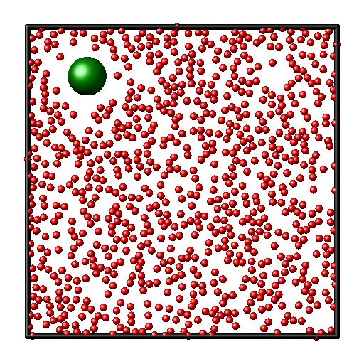
The simulation is identical to the above, except that one large Brownian particle (green) is also present and the density of the solvent particles are somewhat higher than before. Due to collisions with the solvent the brownian particle is randomly kicked around and executes a random walk. Try changing the mass or size of the particle, you can also add more brownian particles. You can also try download brownian_langevin.lam. Here the solvent is replaced by a Langevin dynamics where the particle feels a stochastic kick and a friction force modelling the effects of the solvent. This is an implicit solvent model, and it runs many times faster than the simulation where the solvent is modeled explicitly.
Lennard-Jones liquid
Download lj.lam and put it in a folder. Start a command shell and run lmp_serial -in lj.lam in the folder where you saved cryst.lam. After the simulation is completed you can look at the JPEG pictures in the img folder or play the movie.avi.
 |
|

The Lennard-Jones potential models the attraction between noble gas atoms due to dispersion interactions. It is strongly repulsive at short distances, but attractive at intermediate distances. This system was studied with Molecular Dynamics techniques back in 1967 by "Computer "Experiments" on Classical Fluids. I. Thermodynamical Properties of Lennard-Jones Molecules" Loup Verlet Phys. Rev. 159, 98 (1967). The Langevin thermostat adds a friction on each particle that extract heat from the system, but it also adds a random force kick to each particle that injects heat into the system. The combined effect models the system being in contact with a heat bath with a specified temperature. Try playing with the density and temperature and see what phases you get. During the simulation the radial distribution function is sampled which is shown to the right, which shows the typical shell structure of a dense liquid. Try plotting the lj.rdf file for various phases (column 2 is radial distance, column 3 is the probability of particles at this distance).
Melting a crystaline LJ cluster
Download cryst.lam and put it in a folder. Start a command shell and run lmp_serial -in cryst.lam in the folder where you saved cryst.lam. After the simulation is completed you can look at the JPEG pictures in the img folder or play the movie.avi.
500 particles are put into the middle of a 2D box with periodic boundaries. These particles interact via a Lennard-Jones potential. At T=0 the particles are in a crystalline state, at T=0.5 they melt into a diffuse liquid droplet, if you heat it further it turns into a gas. Try to change the number of particles, or the start and end temperatures!
|
T=0 |
T=0.5 |


Demixing
Create a folder e.g. demix under your user folder. Download demix.lam andput it in that folder. and run a simulation with lmp_serial -in demix.lam

The simulation comprises 12000 red and 12000 green particles. Initially these are randomly dispersed, but since red likes red and green likes green, but they red and green particles dislikes each other, the system undergoes a spinodal decomposition process, until there is just a single droplet, hence minimizing the surface energy. This model uses Dissipative Particle Dynamics, which can be directly related to regular solution theory. For the choice of interaction parameters shown chi=15.7, which is above the critical chi=2 and we see the system phase separates.
Polymer dynamics
Create a folder e.g. poly under your user folder. Download poly.lam and the input file poly1.input put it in that folder. Start a command shell, navigate to the poly folder (command cd poly), and run lmp_serial -in poly.lam . After the simulation is completed you can look at the JPEG pictures in the img folder or play the movie.avi.
|
|
|
|


A polymer is a linear molecule, here modelled as 40 particles that are bonded to each other. The dynamics is Langevin, i.e. each particles feels the bond forces from the neighboring particles as well as a friction and a stochastic kick modelling a temperature of 3 in reduced units. In the simulation, the polymer is not allowed to cross itself. The dynamics of a single polymer is known as Rouse Dynamics, the polymer wiggles around due to thermal fluctuations. Try playing with the temperature and see what happens. Alternatively, you can add constraints. In 2D these green particles are fixed and the polymer is not allowed to cross them. In 3D the constraints would be due to other polymers forming a network. In the simulation these constraints do not move, and since the polymer can not cross them, the thermal fluctuations of the polymer is now localized to a tube along the polymer. This dynamics is called Reptation motion, because like a snake the polymer can only move by slithering along the constraints. Understanding the properties of the tube and the reptation dynamics is the basis for understanding the elasticity of rubber and viscoelastic behaviour of gels. Try playing with the number of constraints and see what happens. If you want more than one polymer, download the input file poly5.input. Finally, try adding a force to the polymers and look at how they move through the obstacles. You need to find and unremark a line in the poly.lam file for doing this. Pulling polymers through a gel is known as electrophoresis, and is used e.g. to size sort DNA molecules.
Polymers can made made in all kinds of molecular structures. If you want to try other molecular structures, try downloading poly1-circle.input or poly1-star.input . The circle consists of 60 beads. The star has 4 arms of length 20 beads. With obstacles these molecules shows a completely different dynamics than the linear polymers.
Rouse model of Polyethylene chain
Create a folder e.g. pe300 under your user folder. Download pe.lam and the input file poly5.input put it in that folder. Start a command shell, navigate to the pe300 folder (command cd pe300), and run lmp_serial -in pe.lam . After the simulation is completed you can look at the JPEG pictures in the img folder or play the movie.avi.

This setup performs a short simulation of 5 chains of polyethylene molecules of Mw=10^4 g/mol. This corresponds to a harmonic spring model with 216 springs where the mean-square extension of each spring is Sqrt(<b^2>)=2.55Å. This is realized by using harmonic bonds with k=0.275Kcal/mol =19.1pN/Å. This setup uses real units rather than LJ units. The box size is 100x100x100Å and the end-to-end distance is sqrt(<R^2>)=Sqrt(1400Å^2)=37Å which is about 1/3 of the box size in good agreement with the picture.
Polymer being pulled by external force
Create a folder e.g. poly under your user folder. Download pull.lam and the input file poly1.input put it in that folder. Start a command shell, navigate to the poly folder (command cd poly), and run lmp_serial -in pull.lam . After the simulation is completed you can look at the JPEG pictures in the img folder or play the movie.mpg.
 |
 |
The polymer is tethered to the wall and a force is applied to the free end. The polymer consists of 40 particles (39 bonds). Compared to the polyethylene model above, the present simulation use FENE bonds rather than harmonic bonds, since this bond potential model the finite extensibility of real polymer chains. During the simulation the external force increase as a linear function of time. During the simulation the average end-to-end distance along the x axis is measured. The plot shows this end-to-end distance (xaxis) and the imposed force (yaxis). The stronger than linear response (which we would expect from harmonic spring) is the hallmark of finite-chain extensibility effects.
Uniaxial / Shear deformation of network
Create a folder e.g. network under your user folder. Download network.lam and and the input file network.input put it in that folder. Start a command shell, navigate to the network folder (command cd network), and run lmp_serial -in network.lam . After the simulation is completed you can look at the JPEG pictures in the img folder or play the movie.avi.
 |
|

The script can both shear and uniaxially deform a network of springs. The two renderings shows the final states. Before, during and after the deformation you can sample the shear strain vs. shear stress or elongation vs. normal stress and make plots of how these evolve with time.
Shear relaxation of polymer liquid
Create a folder e.g. dumbbell under your user folder. Download dumbbell.lam and put it in that folder. Start a command shell, navigate to the percolation folder (command cd dumbbell), and run lmp_serial -in dumbbell.lam . After the simulation is completed you can look at the JPEG pictures in the img folder or play the movie.avi.

In this script 200 spring polymers of length 100 is put into the simulation domain.The script samples the shear stress before, during and after a rapid shear step deformation. The rapidly deformation gives rise to a peak in the shear stress, however, since this is a liquid it can not sustain a permanent stress, and we observe a rapid decay of the shear stress to zero.
Percolation
Create a folder e.g. percolation under your user folder. Download porcolation.lam and put it in that folder. Start a command shell, navigate to the percolation folder (command cd percolation), and run lmp_serial -in percolation.lam . After the simulation is completed you can look at the JPEG pictures in the img folder or play the movie.avi.

In this simulation an initial gas of 350 particles can form bonds with each other when they are within a certain capture radius.The particles rapidly forms a network spanning the system, i.e. models a percolation process. Particles are limited to having maximally 3 bonds, which has a strong influence on the network structure. When bonds are added, angular interactions are also created such that the resulting chains are rigid and filamentous rather than random walks. Try playing with the density of particles, maximum functionality, probability of making a bonds, or rigidity to see what percolation networks are formed.